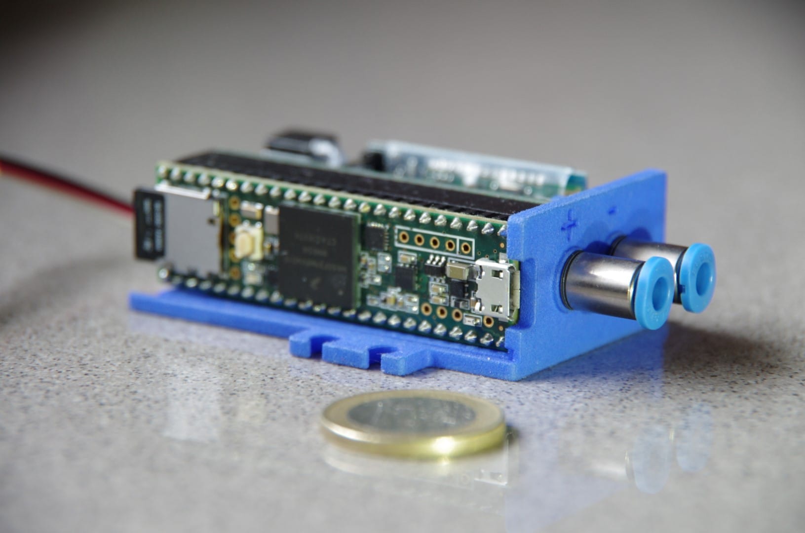
The air data computer Asgard is out. It is a unit designed for DIYers, size and weight are compatible (fixation tabs have the same dimensions of standards servo tabs) with low-cost RC applications. Some aspects will be changed as per users feedback. Be sure to checkout the project website for detailed information on how you can build your own.
Some time ago we presented a free software mini-suite that can be useful to support UAV based survey tasks/general purpose operations.
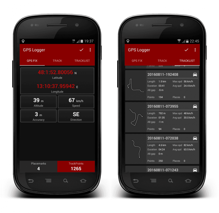
The new Basic Air Data GSP Logger App release was tested at Centre for Geoinformatics, IIFM, Bhopal, India; the results were as expected.
They produced a pdf report and 15 minutes quick start up video-tutorial for GPSLogger. The pdf report contains the details about GPS Logger altitude correction.
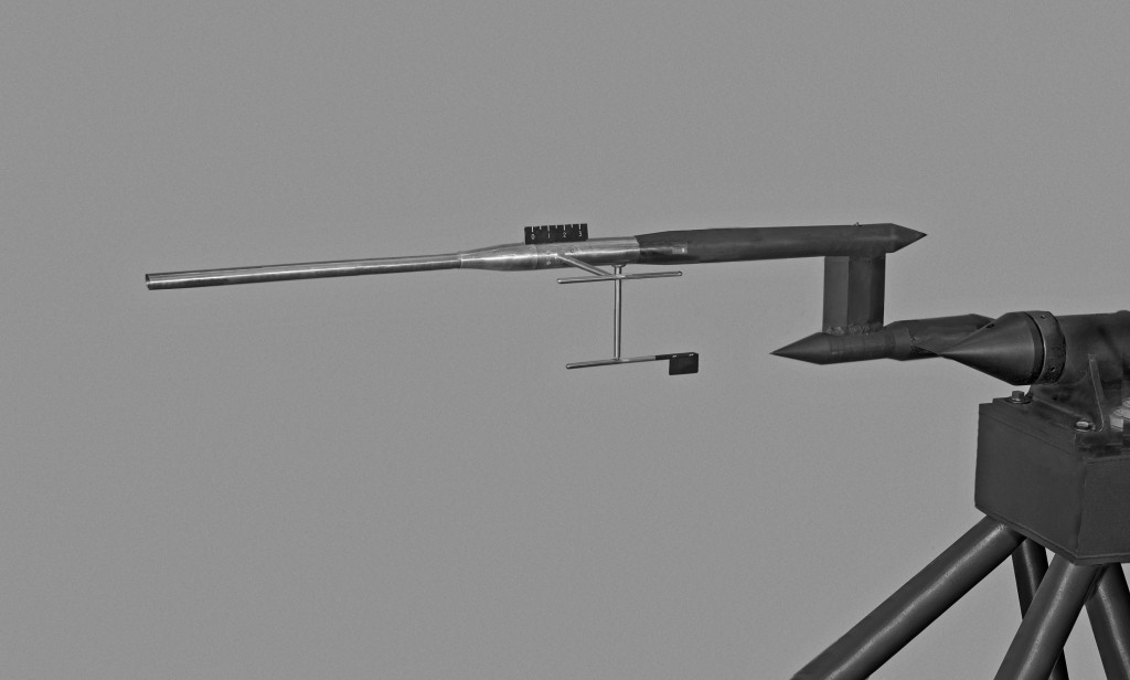
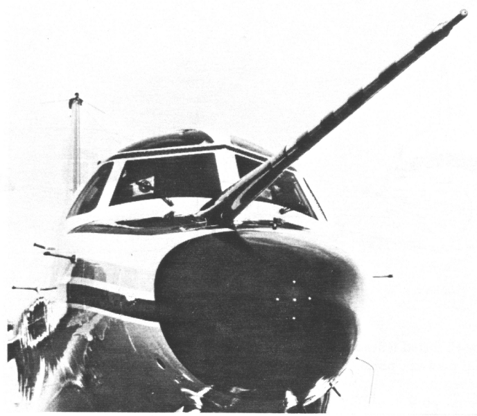
Figure 1: Mechanical Air Data Boom tested in 4x4 tunnel
Air data can be acquired by mean of mechanical probes protruding from the airframe. In many cases was also possible to find a placement for the probe that is out of the body modified airfield. Very common is the nose mounted air data boom. In Figure 1 you find one mechanical air data boom tested within a wind tunnel in 1958 (Source: NASA).
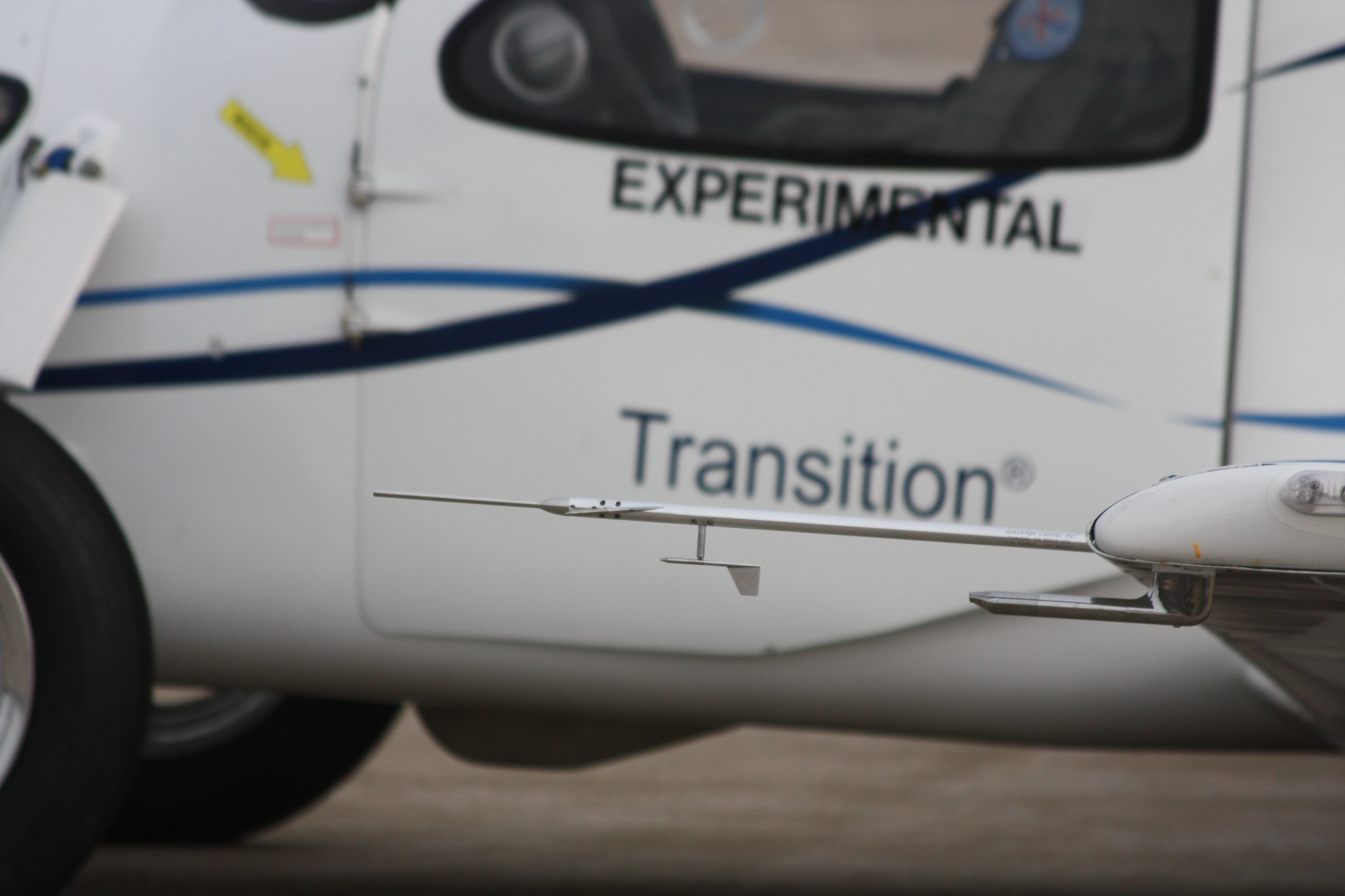
Mechanical Air Data Booms are able to reach a notable degree of accuracy and are used in some modern applications, you see a miniature mechanical Air Data Boom mounted on the Terrafugia prototype in Figure 2.
Figure 2: SpaceAge Control miniature 100400 Air Data Boom
Apart the weight and the size, this solution should deal with its intrinsic mechanical nature, mechanical-friction, inertia and robustness consideration are of high impact on overall probe design and performances. Mechanical related problems are exalted in both at low and high airspeed. At low airspeed, we have a low aerodynamic force to win the wind vanes frictions. At high airspeed, the aerodynamic damp of the wind vane will decrease and can lead to an unacceptable dynamic behavior. Anyway, an alternative to the classical probes is to reconstruct wind direction using multiple pressure readings. That defines two big families of probes the first is the so-called Multi Holes Probes and the second the Flush Airdata Sensors.
Figure 3: Aeroprobe ADC with 6 holes MHP
With a classical probe, the information on wind direction is available directly from the two wind vanes angular sensors signal, in a pressure based system that information should be reconstructed from different pressure readings. Refer for example to the commercial MHP of Figure 3. On this probe tip, there are presents six different pressure ports. There is a central hole that can give exactly the same pressure reading of that measured by the total pressure hole of a Pitot-Static probe. There is an annular pressure port, at a certain distance from the probe tip, that measures the static pressure; in a similar way of the Pitot-Static probe static port. There are 4 supplementary holes on the probe head. They can be used, for example, but not only, in couples to determine the angle of attack and the angle of sideslip. Data reduction algorithms can use the combined data from all the six pressure taps to reconstruct
\(P_t\) Total pressure or impact pressure \(P_s\) Static pressure \(\alpha\) Angle of attack \(\beta\) Angle of sideslip
The pressure at ports is correlated to the relative wind magnitude and direction, you find a developed example of the angle of attack measurement case in this link. This kind of probes is used usually in many research and industry fields, including turbomachinery. MHP probes can reach dimensions under the 6 mm diameter.
FADS are similar under many aspects to MHP but the probe surface is usually one airframe surface exposed directly to the air stream. In many cases, the sensor openings are over a modified nose cone. Refer to Figure 4, here you find a FADS system; description of the system here.
Figure 4: NCAR Sabreliner aircraft equipped with both the differential pressure probe and the radome with pressure ports
This kind of probe is commonly used in research applications. Many studies were conducted by Langley NASA research center for the shuttle space program [page 6]. Dryden Flight Research center continued the work and produced different interesting articles. You can find notable information within this NASA work or in this work on X-33 FADS. Regarding real time data reduction consideration please consider that other article.
Both the families of probes can reach notable performances. Calibration, both aerodynamic and of single pressure sensors, and reduction algorithms for the FADS can pose a more that respectable practical problem. I've no notice, to date, of any DIY probe of that kind. It is to be noted that DIY aircraft have reduced flight speeds, that signifies that magnitude of pressures measured or differential measured differential pressure is really of small value; for a medium demanding application, we may need to have pressure measurements accurate to about a Pa. It's clear that an extremely well-calibrated measurement hardware is needed. It seems neither easy nor cheap to go under one degree of overall accuracy on AOA measurement. As many users are interested in the topic we will develop it in time and publish the results online. For the same reason if you think you can contribute to development please enter in contact with us.
Here I share one of the tested DIY designs from BasicAirData
Our most popular 8mm pitot flangeuses two 3D printed barbed nipples as connectors for pneumatic lines. That design is functional, yet the user is required to drill holes in the nipples with a 1mm drill, which can be quite a task. To alleviate that burden, we decided to produce a new nipple design, with the code-name Zen. The resulting flange is also easier to 3D print.
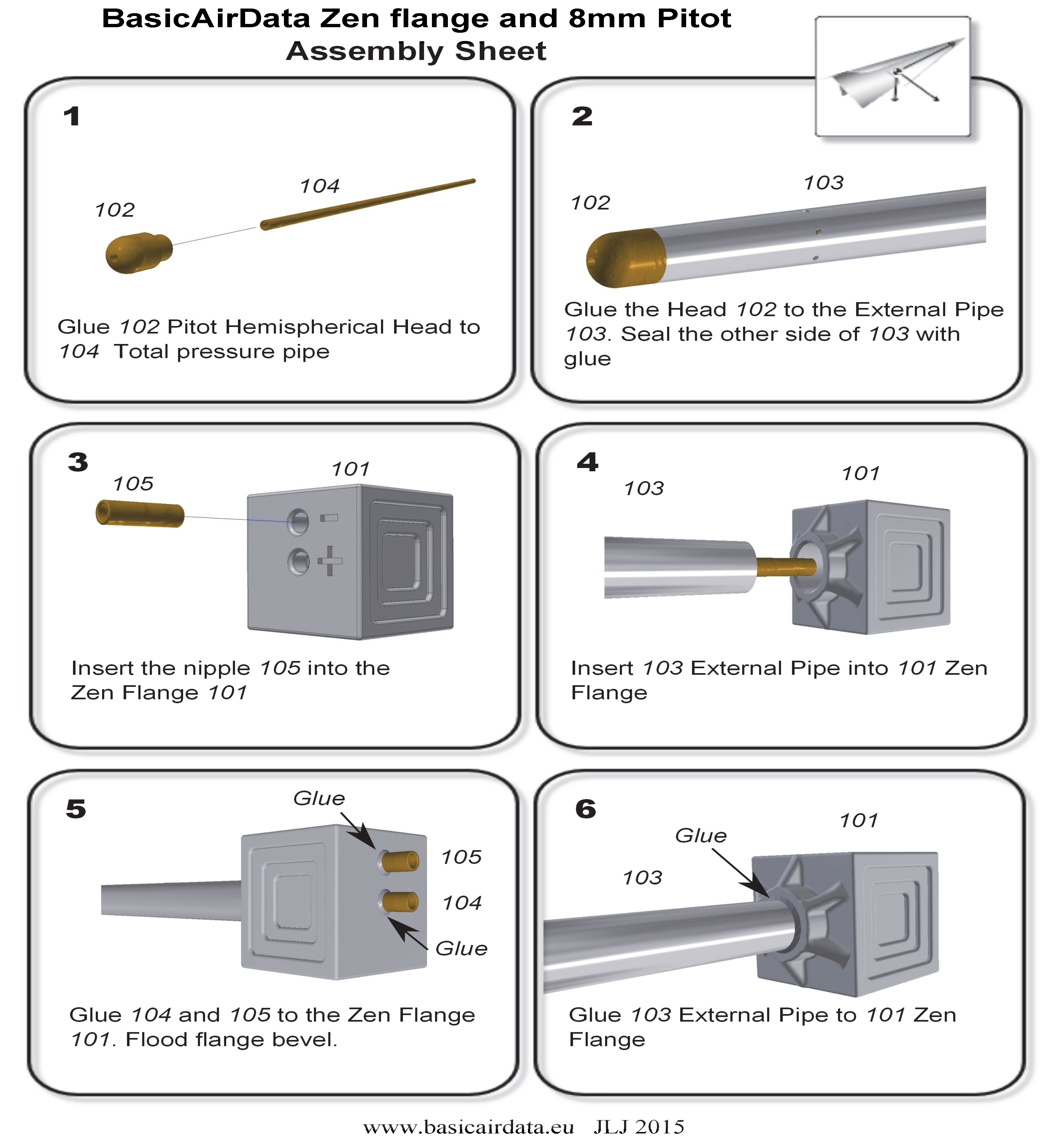
The assembly is fast and revolves around a signle 3D printed part (STL file). An assembly cheat-sheet can be seen in Figure 2.
Figure 2: Assembly Sheet
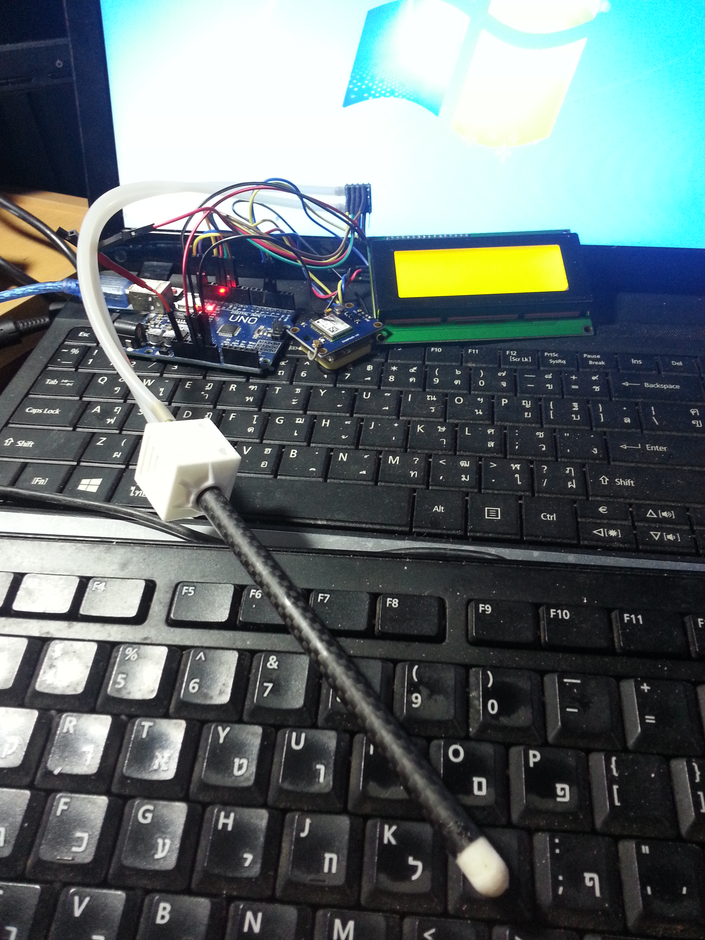
Figure 3: Printed Zen Flange
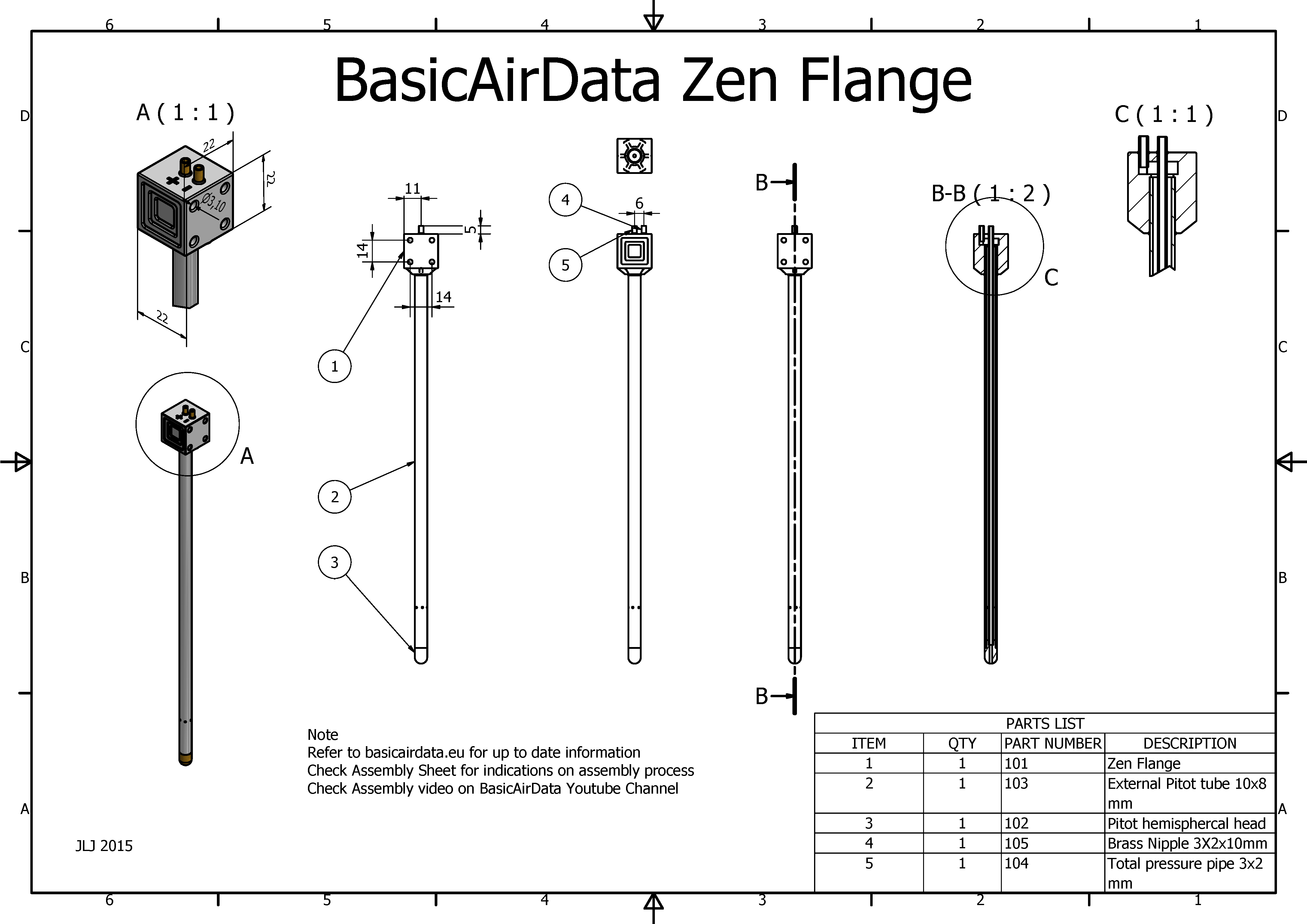
The assembly procedure doesn't consist but of trimming three tubes and gluing the whole thing together. Let the overall length of your probe be L(mm), in our example L=200. The overall length is defined as the distance from the tip of the probe to the back of the flange, excluding the nipples.
The external pipe has an outer diameter of 8mm and an inner diameter of 6mm. A carbon fiber tube is a good choice. Trim it at L-18mm, which is 182mm in our example.
Drill the static pressure ports on the outer pipe, at a distance of 36mm from the front pipe end. Drill 8 holes of 1mm diameter, 45° apart. This procedure is identical to our previous probe model.
Cut a nipple of length of 10mm (refer to assembly sheet item 105), for example out of a brass tube, with outer diameter of 3mm and inner diameter of 2mm.
Cut the total pressure pipe (item 104) at a length of L-7mm (193mm in our case), for example out of a brass tube, with outer diameter of 3mm and inner diameter of 2mm.
Figure 4: Rendered Section View
Video 1: Assembly Test Video
When you have prepared all the parts, make a little assembly check as per Video 1.
After a positive assembly check you can glue the pieces together. The important interface is that between the Pitot head (102) and the total pressure pipe (104). It is critical that this glue seal is airtight. Once you glue the external pipe (103) on the Pitot head you will not be able to repair any leaks.
Once you have glued all the parts together, you should test if the two pneumatic paths are free of obstacles and airtight. If it is available, a Pitot-static tester can be used. If not you can perform a quick test by following this simple procedure:
Blow into the + nipple. The air should flow unobstructed down to the total pressure port.
Seal the total pressure port with your finger and blow into the + hole. There should be no air leaks.
Blow into the - nipple. The air should flow unobstructed down to the static pressure ports.
Seal the static pressure ports with adhesive tape and blow into the - hole. There should be no leaks.
So far, the pneumatic connections on our Pitot-static system were considered perfectly airtight. For a change, in this article we examine typical leakage scenarios and their impact on airspeed and altitude measurements. We will focus on leakage solely in the static system; study of the leakage in static pressure piping is important, since at high airspeeds, deviation in static pressure will lead to airspeed measurement errors. Perhaps in the future we will be able to dedicate some time on leakage on the total pressure port as well. In this article, our approach will be to use a lumped parameters leakage model to get preliminary results on the behaviour of our system under leak conditions... [Read more]
NOTE : Experimental. To avoid formulas visualization issues we've setup a free Newsletter. Once subscribed you will receive a pdf with the article. http://www.basicairdata.eu/newsletter.html
In this short article we will make an effort to calculate the flow rate of a volume of air via \(n\) multiple velocity measurements at a selected pipe section. Velocity profiles are useful when evaluating small DIY wind tunnels and nozzle designs. Although this article doesn't reflect any particular technology, the reader can imagine that velocity measurements themselves are carried out with a Pitot tube or with a Pitot rake placed at the section in question. There are different industrial standards that cover the topic, such as the ISO 3966: Measurement of fluid flow in closed conduits - Velocity area method using Pitot static tubes. In the following test we will not follow any particular standard. Still, those standards are interesting readings.
We are interested in calculating the volumetric flow rate, \(Q\). The volumetric flow rate is the volume \(\Delta V\) that flows across a predefined surface in an arbitrary interval of time \(\Delta t\), \(Q=\frac{\Delta V}{\Delta t}\).
Figure 1 - Sectioned pipe and flowing fluid
Refer to Figure 1; A section perpendicular to the pipe axis defines a circular surface of area\(s\). On the assumption that the axial velocity at every point of the section is constant and equal to \(V_c\), then \(Q=V_c\cdot s\). An animation of the system at hand can be seen in the following video
Video 1 - Volumetric Flow rate
The fluid velocity is constant over the section and time. A flow rate of 4.4e-6 \(m^3/s\) is equal to the red cylinder volume, 13.2e-6 \(m^3\), divided by the transit time through the section plane, 3\(s\).
However, in the real world the velocity is not constant across the section. The interaction of the fluid with the pipe surface generates a non-negligible velocity gradient. In general, it stands that \(Q=\int v(x,y,)dt\). Bibliography comes handy and we will use a power-law velocity profile. With this model, we will build a reference pipe numerical model, which represents the pipe and the flow rate which we will measure. The real-world pipe is replaced by a numeric simulation. The commonly used model does not separate the viscous sublayer nor the transition layer; in fact it is discontinuous at the surface of the pipe and on the symmetry axis. Since we are not treating a particular real-word case we're not concerned about the uncertainty introduced by the power-law model. Details about the viscous sublayer and the transition layer can be found in this link.
We end up using a fully developed turbulent axial flow model at high Reynolds number. The viscous layer is expected to be thin in typical cases (like a hair) and it is not calculated in this example. You can find a Scilab script in this file that will calculate the power-law velocity profile for you. The result is visible in the next figure.
The resulting velocity profile is dependent solely on the distance from the axis. You can see that the velocity gradient, as expected, is high near the pipe wall and low along the center line.
Now it is time to measure the flow rate. Refer to Figure 3. We assume having access to velocity measurements at \(n\) stations. Each station is at a different distance \(r(n)\) from the pipe center line. For the sake of simplicity, we divide the radius in \(n\) equal segments. For each segment we measure the velocity \(v(n)\) at its midpoint.
Figure 3 - Velocity measurements position into the measurement section
We make the assumption that the velocity remains constant along each segment of the radius and, by extension due to axial symmetry, over the whole corresponding annular ring. The total volume that passes through the ring surface is the product of velocity with the annulus area. Iterating the calculation for all the segments we calculate the volumetric flow rate as \[Q=\sum_{i=1}^n v(n)\pi(r_{ext}^2(n)+r_{int}^2(n))\], where
\(i\) is the annular ring index
\(v(n)\) is the velocity of \(i\) ring
\(r_{ext}\) is the outer ring radius of \(n\) ring
\(r_{int}\) is the inner ring radius of \(n\) ring
Figure 4 - Velocity profile reconstructed by 10 measurements
Figure 4 visualizes the velocity profile as reconstructed by our measurements. It is evident from the profile steps that we have a coarse approximation. There is a simple way to get better flow rate measurements: we can use the model to calculate the velocity profile within each annulus. In such a way, using our simulation data, we will get exactly the flow rate produced by our reference model. Driven by this result, we can even try to use only the data from one single measurement, for example at the center line. Doing so we will bring the very same result predicted by our reference model. Unfortunately the accuracy is constrained to the ability of the model to capture the real world with all accuracy. For that reason, in actual applications, in general, the accuracy should be expected to be higher when using multiple simultaneous measurements rather than model interpolations. But let's leave this problem to the professionals, for now.
In this article we have explored the basics of volumetric flow rate measurement with the velocity-area method. This topic is quite relevant to basic air data processing because it shows the impact of the flow pattern on simple calibration instruments like small size / DIY size wind tunnels.
NOTE : Experimental. To avoid formulas visualization issues we've setup a free Newsletter. Once subscribed you will receive a pdf with the article. http://www.basicairdata.eu/newsletter.html
Air density \(\rho\) is a common case of measurement derived from air data. Let's investigate the relationship between air temperature and air density, which, incidentally, is the base of the external air temperature measurement in moving vehicles.
Commonly the air density can be calculated with an equation of state or with an interpolated best-fit curve. In both cases, we have to deal with an equation of the form \(\rho=f(T,p,RH, others)\). Let's make things a bit simpler and start with a simple relationship between density and temperature:
$$\rho=f(T,Constant)$$
Temperature in the SI is measured in degrees Kelvin, but many equations of state may also be given with temperature expressed in \(Celsius=Kelvin – 273.15\). Quoted from BIMP: "The kelvin, unit of thermodynamic temperature, is the fraction 1/273.16 of the thermodynamic temperature of the triple point of water.". The thermodynamic temperature is correlated to the state of a thermodynamic system and according to the third law of thermodynamics it defines an absolute temperature scale. For dry air, the ideal gas equation of state is
$$\rho=\frac{p}{R_{specific}T}$$
where
\(\rho\) is the air density in \(kg/m^3\),
\(p\) is the absolute pressure in \(Pa\),
\(T\) is the absolute temperature in \(K\) and
\(R_{specific}=287.058\frac{J}{kgK}\) is the specific gas constant for air.
The main advantage of the equation of state is that it provides a closed form solution, which in turn can be incorporated in other computations. This is a very convenient property for analysis purposes. Let's proceed with a density calculation. Refer to figure 1; our idealized test setup is a room with two thermometers and a fan. The first thermometer measures the temperature of the air in the room at a point far away from the fan effects, while the second one is subject to the direct airflow from the fan.
Figure 1: Example layout
Prior to any calculation let's introduce the stagnation temperature, which indicates the temperature at a stagnation point within a flow field. At the stagnation point the local flow velocity is zero. We find a stagnation point on a Pitot tube tip or in a total air temperature probe.
In our example, the air from the fan which hits the thermometer is brought to rest on the surface of the sensing element. Consider an infinitesimal volume of the overall air stream traveling at a certain speed. This small volume has a corresponding kinetic and gravitational potential energy. If we assume that this volume does not exchange any form of energy with the surroundings then this energy must be converted when one of its forms is eliminated. In the process where the air slows down, kinetic energy is converted into heat, which causes a temperature rise. Assuming an adiabatic process we can describe the enthalpy at stagnation
$$h_s=h+\frac{V^2}{2}$$
where the enthalpy term \(h\) is that of the nearest point along the streamline and
\(V\) is the speed of the air flow.
For an ideal gas it holds that
$$h=u+pv$$
where \(v\) is the specific volume and
\(u\) is the internal energy of the gas.
By manipulating the enthalpy expression and taking into account the constant pressure heat capacity definition \(Cp\) for an ideal gas \(h=C_pT\), we arrive at
$$T_s=T+\frac{V^2}{2C_p}$$
This equation defines how much the temperature rises because of the fact that is adiabatically brought to rest.
Returning to our example let's calculate the different values of stagnation temperature in correspondence of different airspeed values. You can find pre-calculated values in the table below.
T [K] Static
V [m/s]
V [km/h]
M
T0 [K] Stagnation
Deviation [K]
Deviation [%]
Parameters
288.15
0
0
0
288.15
0
0
Cp
1005
J/Kg/K
288.15
2
7.2
0.01
288.15
0
0
c
340.3
m/s
288.15
3
10.8
0.01
288.15
0
0
288.15
4
14.4
0.01
288.16
-0.01
0
288.15
5
18
0.01
288.16
-0.01
0
288.15
6
21.6
0.02
288.17
-0.02
0.01
288.15
7
25.2
0.02
288.17
-0.02
0.01
288.15
8
28.8
0.02
288.18
-0.03
0.01
288.15
9
32.4
0.03
288.19
-0.04
0.01
288.15
10
36
0.03
288.2
-0.05
0.02
288.15
11
39.6
0.03
288.21
-0.06
0.02
288.15
12
43.2
0.04
288.22
-0.07
0.02
288.15
13
46.8
0.04
288.23
-0.08
0.03
288.15
14
50.4
0.04
288.25
-0.1
0.03
288.15
15
54
0.04
288.26
-0.11
0.04
288.15
16
57.6
0.05
288.28
-0.13
0.04
288.15
17
61.2
0.05
288.29
-0.14
0.05
288.15
18
64.8
0.05
288.31
-0.16
0.06
288.15
19
68.4
0.06
288.33
-0.18
0.06
288.15
20
72
0.06
288.35
-0.2
0.07
288.15
21
75.6
0.06
288.37
-0.22
0.08
288.15
22
79.2
0.06
288.39
-0.24
0.08
288.15
23
82.8
0.07
288.41
-0.26
0.09
288.15
24
86.4
0.07
288.44
-0.29
0.1
288.15
25
90
0.07
288.46
-0.31
0.11
288.15
26
93.6
0.08
288.49
-0.34
0.12
288.15
27
97.2
0.08
288.51
-0.36
0.13
288.15
28
100.8
0.08
288.54
-0.39
0.14
288.15
29
104.4
0.09
288.57
-0.42
0.15
288.15
30
108
0.09
288.6
-0.45
0.16
288.15
31
111.6
0.09
288.63
-0.48
0.17
288.15
32
115.2
0.09
288.66
-0.51
0.18
288.15
33
118.8
0.1
288.69
-0.54
0.19
288.15
34
122.4
0.1
288.73
-0.58
0.2
288.15
35
126
0.1
288.76
-0.61
0.21
288.15
36
129.6
0.11
288.79
-0.64
0.22
288.15
37
133.2
0.11
288.83
-0.68
0.24
288.15
38
136.8
0.11
288.87
-0.72
0.25
288.15
39
140.4
0.11
288.91
-0.76
0.26
288.15
40
144
0.12
288.95
-0.8
0.28
288.15
41
147.6
0.12
288.99
-0.84
0.29
288.15
42
151.2
0.12
289.03
-0.88
0.3
288.15
43
154.8
0.13
289.07
-0.92
0.32
288.15
44
158.4
0.13
289.11
-0.96
0.33
288.15
45
162
0.13
289.16
-1.01
0.35
288.15
46
165.6
0.14
289.2
-1.05
0.37
288.15
47
169.2
0.14
289.25
-1.1
0.38
288.15
48
172.8
0.14
289.3
-1.15
0.4
288.15
49
176.4
0.14
289.34
-1.19
0.41
288.15
50
180
0.15
289.39
-1.24
0.43
288.15
51
183.6
0.15
289.44
-1.29
0.45
288.15
52
187.2
0.15
289.5
-1.35
0.47
288.15
53
190.8
0.16
289.55
-1.4
0.48
288.15
54
194.4
0.16
289.6
-1.45
0.5
288.15
55
198
0.16
289.65
-1.5
0.52
Table 1. Stagnation temperature vs static temperature at different V values. Download spreadsheet.
By inspection of the table, the deviation between the two temperature measurements increases with the air speed.
The air density in the room should be calculated using the static temperature, in our case, for e.g. \(p=101325 Pa\) the corresponding density is \(\rho=1.225\ kg/m^3\). The same calculation using the total temperature with a fan pushing the air at 55 m/s gives \(\rho=1.218\ kg/m^3\), which is about a 0.5% of error on density.
Inspect the relationship between static and total temperature for a total air temperature probe; the first formula in this link.
$$T_{total}/T_s=1+\frac{\gamma-1}{2}M^2$$
where the “total” subscript indicates the adiabatic temperature and “s” subscript is for the static temperature. This formula is in accordance with our example formula. To reach this formula from our derived temperature equation, substitute in this formula the definition of the specific heat ratio \(\gamma=C_p/C_v\), the Mayer's relation \(C_p – C_v = R\) and the Mach number expression \(M=V/\sqrt{\gamma R_{specific}T}\).
The total air temperature computed up to now here is somewhat ideal. All the kinetic energy is converted and contributes to a temperature rise but it should be accounted with an appropriate recovery factor (Commercial example here, equation 3). The relationship of the recovery factor with airspeed and other environmental factors is not trivial and for best accuracy it should be experimentally found. Nonetheless, the tight relationship between airspeed and temperature can be exploited to have a true air speed indication as per equation 9 in the previous link. Consequently, a total air temperature probe working together with a Pitot-static tube offers a useful redundant airspeed indication.
Even at low airspeeds, to achieve top performance, the temperature measurement rise due to airspeed is existent. However, the impact of this effect on temperature measurements can be neglected in many applications with moderate to no loss of accuracy. Unfortunately, this is not the only source of uncertainty in a total air temperature probe. There are other aspects that hinder much more the performance of the total air temperature probes. Thermal aspects will be considered in a following article.
The Reynolds number can be used to predict a flow pattern. The onset of very fascinating flow patterns, for example vortex streets (Tutorial here) can be detected with the use of Reynolds numbers.
The Reynolds number is the ratio between inertial and viscous forces. A low Reynolds number indicates that inertial forces are overwhelmed by viscous forces. Conversely a high Reynolds number indicates that inertial forces are driving the flow. We can distinguish three principal flow patterns: laminar, transitional and turbulent.
We have a laminar flow when the fluid flows in parallel layers, each layer having little interaction with the adjacent layer. In a laminar flow it is possible to distinguish parallel flowing streamlines. An extreme example of laminar flow is shown on the following video.
Video 1 - Laminar flow twisting and untwisting
This flow has a very low Reynolds number, well below unity. As the flow is strongly laminar the operator can rewind the system to a state visually identical to the original state
Turbulent flow is characterized by an apparent randomness, circulation, eddies and high Reynolds number.
A transitional flow is somewhat in between the two previous cases: some parts of the fluid can have a laminar behavior and some others a turbulent-like behavior. Determining the Reynolds number for each pattern in the transtional flow is not trivial, but fortunately for many notable cases there is an approximate math model. In the next video a complete transition between laminar and turbulent flow into a pipe is shown.
Video 2 – Transition between patterns
In the relevant literature, one of the most well-studied boundary layer patterns is the one formed by a flow over a flat plate. Under some assumptions, the boundary layer expression can be analytically found, for example there is the Blasius solution. Have a look at Figure 1. One important thing to observe is that the boundary layer is developing along the plate \(x\) coordinate, on the horizontal direction of the image. The Reynolds number expression is \(Re=\rho Ux/\mu\) and \(x=0\) corresponds to the leading edge of the plate or the beginning of the boundary layer itself. Initially, the flow is laminar and as \(x\) increases the Reynolds number increases as well. At some point, the boundary layer transforms into a transitional pattern and finally ends with a turbulent configuration. If one is able to increase \(x\) at will, the flow will become turbulent sooner or later. Depending on many factors, like fluid type and plate roughness the transition to turbulent flow will happen at a different Reynolds number. A plausible interval of values is from 1e5 to 3e6.
Figure 1 – Boundary layer over a flat plate
The larger the x-coordinate of the section we examine is, the wider the corresponding boundary layer will be. Given a section at a coordinate \(x\), we observe that the thickness of the corresponding boundary layer decreases as the free stream speed increases. We can observe the relationship between freestream speed and boundary layer thickness on the following video.
Video 3 - Boundary layer experiment water tube
In the video, the transition to turbulent pattern is triggered by an aerodynamic obstacle. Pressure gradients can cause transitions of boundary layers. Pressure gradients are likely to occur on external air temperature probes inside the diffuser section. You can see the geometry of a Kiel probe here.
In the general case, boundary layer shape is time and position dependent and thus no overall closed form solution is available.
In the next article we will investigate in more detail the simplest ways that pressure gradients affect boundary layers and we will examine a numerical example.
Figure 1 – Lovely Heidelberg. I've been there. Birthplace of the boundary layer
When a body moves through the air, its interaction with the surrounding air mass generates a region where the air conditions are different from the freestream conditions. This region is named boundary layer. In basic air data applications there is a need to make accurate freestream conditions measurements, so we're really concerned about boundary layers. Boundary layers have been studied since the very beginning of aerodynamics. In 1904 a twenty-nine-year-old Ludwig Prandtl laid down the groundwork for modern aerodynamics with a short boundary layer presentation in Heidelberg [1].
Let's visualize the boundary layer over a flat plate, refer to Figure 2. We have depicted a laminar air flow, with vectors highlighting the velocity profile. The air flowing near the wall is slower than the air far from the wall, so the local velocity \(u(y)\) is a function of the distance from wall \(y\). The boundary layer is defined as the region where the local velocity values \(u(y)\) are less or equal than the 99% value(or other reference value) of the freestream value \(u_{infty}\). The speed at the wall is zero.
Air is viscous so to move one air layer with respect to other is necessary to apply a force. Let's consider the flow (Couette flow) between two parallel flat plates of area \(A\) at a distance \(y\), one fixed to the ground and the other free to move. The force \(F\) needed to maintain the speed \(u\) of the moving plate is \(F=\mu Au/y\). The newly introduced parameter \(\mu\) is the air dynamic viscosity, with SI unit of measurement the \(Pa \cdot s\). It is evident that energy is required to maintain a boundary layer of given characteristics between the two plates.
Video 1 – Turbulent and laminar flow
IIn general, boundary layers are affected by the relative speed of the fluid, the fluid properties and body geometry; see the following video that visualizes an example of laminar and turbulent flow.
Figure 3 - Boundary layer velocity profiles in CFD pipe
The simplest way to visualize a boundary layer is to run a CFD simulation of a tube. You can find a tutorial here. From the figure 3 it is evident that the boundary layer is present and changes its shape along the pipe, the boundary changes along the length of the pipe, so the flow is said to be developing along the longitudinal axis. Let's suppose we want to calculate the flowrate across the pipe measuring the speed of the fluid at a single point inside the pipe. Flowrate is the integral over time of the velocity across a fixed section multiplied by the fluid density (Eq 12.2). To reconstruct the velocity values on the whole integration section based on a single measurement we need to know the analytical expression of the velocity profile. In many cases, that information can be gathered from precedent research work. It is evident that if we use the only measured velocity value as mean speed, neglecting the boundary layer, then we get a wrong flowrate measurement value.
Let's change the scenario and suppose that we want to know the true airspeed of a racing car, refer to figure 4. The issue here is that airspeed measured within the boundary layer is lower than the freestream airspeed. How far should our Pitot probe protrude from the car body to work properly? Visit this page for an analytical introductory approach.
Figure 4 – Pitot rake on a race car
At a glance to deal with a boundary layer we need to know
The boundary layer thickness
The boundary layer velocity distribution and flow status: turbulent, laminar or transitional?
Flow development patterns: where will the flow change from laminar to turbulent?
In our typical application we're dealing with a flying platform, where unfortunately the boundary layer characteristics change with the aircraft attitude and airspeed. For example the wing downwash affects all the posterior parts of the fuselage. The magnitude and pattern of the airflow are dependent on the angle of attack.
In the real world it is not trivial to find a position that is not affected by the aircraft attitude. To push the measurement performance further, CFD analysis, wind tunnel studies and in-flight calibration are needed.
Until now we focused our attention to the air velocity field, but the same definition of boundary layer can be used to define a temperature boundary layer. both boundary layers impact on basic air data measurements.
In the next post we will go into detail with a numerical example.
Further readings
[1] John D. Anderson Jr(2005), Ludwig Prandtl's Boundary Layer, December Physics Today 2005
F16 Aerobatic maneuver, Thunderbirds Aerobatic Team
This article is a follow-up on the previously presented results. We will examine the power system of a model airplane from the aspect of reliability. Common equipment configurations will be used as examples.
In a vehicle where the primary power source are electric batteries, the most crucial power consumers are the motor, the avionics and the servos. From now on, for the sake of simplicity, we will refer to the powerplant of the aircraft (which is tasked with producing thrust) as the “thrust” system, whereas the rest of the electric power consumers on the aircraft will be called the “control” system. We will carry out a high level analysis, since too much detail would eventually distract the reader from the most relevant factors.
Refer to Figure 1: our first layout consists of a single battery pack connected to the ESC. Control and thurst are powered by the ESC. Our working hypothesis is that the different failures modes can be considered independent.
Figure 1. Single battery system
Let's select the battery pack reliability value at \(R_p=0.96\) and the reliability value of the ESC at \(R_{ESC}=0.98\). The battery and the ESC should be working at the same time, so for the first layout, the reliability is \(R_{l1}=R_p \cdot R_{ESC}=0.940\). We notice that the overall reliability is lower than the reliability values of each single component. Moreover, our system is not redundant, since the failure of each component causes the failure of the overall system.
Our second layout consists of two independent batteries, one for thrust and one for control. One battery is physically connected to the motor's ESC and the other is connected to a BEC circuit that supplies the control module. Usually, the power related to the thrust system has more capacity and nominal voltage than the control battery.
Figure 2. One battery for thrust, one battery for control
Let's set the reliability value of the battery packs to \(R_p=R_c=0.96\), the reliability value of the ESC to \(R_{ESC}=0.98\) and the reliability of the BEC to \(R_{BEC}=0.98\).
Under nominal system operation, the two batteries, the ESC and the BEC should be operational at the same time. From this aspect, the reliability of the second layout is \(R_{l2}=R_p\cdot R_{ESC}\cdot R_c\cdot R_{BEC}=0.885\). At first, this result seems wrong: Despite having used more equipment, the overall reliability is now lower than the initial 0.940 value from Layout 1. Until now we haven't considered in detail what happens when a part of our system fails and that led us to non-comparable results. In fact, under careful examination, the second layout has extended capabilities. In layout 1 we have a probability \(1-R_{l1}=0.06=6\%\) of a total power loss, and if this unfortunate event happens then we will lose control of the vehicle as well as any ability to safely (crash) land the unit. Revisiting layout 2, we calculate the probability to lose completely the vehicle control. The cases that lead to a catastrophic failure are those that include a simultaneous failure of both the batteries or both the ESC and BEC. The following table presents all such failure cases.
Case #
Battery P
Battery C
ESC
BEC
1
fail
fail
fail
fail
2
fail
fail
ok
fail
3
fail
fail
fail
ok
4
fail
fail
ok
ok
5
fail
fail
fail
fail
6
ok
fail
fail
fail
7
fail
ok
fail
fail
8
ok
ok
fail
fail
Table 1. Failure modes that lead to total power loss equivalent to Layout 1
Combining the probabilities of the cases indicated in the table, we get the following expression for reliability \(R_{l2flat}=1-((1-R_p)\cdot(1-R_c)+(1-R_{ESC})\cdot(1-R_{BEC}))=1-(0.0016+0.0004)=0.998=99.8\%\). Now the odds changed to being favorable to Layout 2. However from a user's point of view, it is more interesting to know the value of the probability that the vehicle is still controllable (at least to some degree) after a failure. The necessary condition for controllability is that the BEC and its battery are still working properly.
Refer to the next table. In cases 9 to 12 the pilot will have a chance to land the aircraft safely.
Case #
Battery P
Battery C
ESC
BEC
9
fail
ok
fail
ok
10
ok
ok
fail
ok
11
fail
ok
ok
ok
12
ok
ok
ok
ok
Table 2. Failure modes that lead to a controllable (crash) land.
The reliability related to this minimum guaranteed performance is \(R_{l2user}=R_c\cdot R_{BEC}=0.940\). This value is the same as the value of the first layout. With this method of analysis, the advantage of layout 2 over layout 1 not so clear anymore. However, the situation can be radically different if there is a relationship between the reliability of batteries/ESC/BEC and the corresponding capacity/max-current/etc or there is a dependency among the reliabilities of single items.
All things said, however, by inspection of layout 2, it is evident that it does not offer any physical redundancy, so statistics apart, it's wise to not expect any sudden reliability increase.
Figure 3. One battery for thrust, dual batteries for control
In this layout number 3, we have a battery that goes straight to the ESC and a redundant voltage regulator, powered by two separated batteries, which feed the control system. The working hypothesis is that the redundant voltage regulator will continue to work even if one battery fails. The most tricky failure to handle for the voltage regulator is a battery cell short. Fortunately even regulators at RC grade can handle this condition [1].
Back to the math, this layout is more reliable as the system composed by voltage regulator with \(R_v=0.98\) and two batteries with \(R_c=0.96\).
Using the same battery pack type, layout 3 offers augmented reliability, and that result was reached by means of physical components redundancy.
Typically, the weakest link in the chain affects the system reliability the most, so prior to purchasing or building an expensive or complex reliable thrust system, an analysis of the reliability of the whole aircraft system should be performed. It will be useless to have an amazing thrust system with undersized servos.
The power system is an essential part of every flying device. If the power system fails then our beloved flying platform will fall out of the sky, and sometimes the damages can even include our calibrated air data instrumentation! The solution is a redundant power system. We will discuss here on the reliability of a range of commonly used power system layouts.
Figure 1- Focke Wulf 3x1000. Redundant power system. The engineer went to great extends to ensure reliability by installing of two independent receivers
Prior to considering the performance of any layout we will first discuss the reliability of a battery pack alone. Battery packs are composed by single cells, connected in series or in parallel. There are different technologies on batteries cells, for example LiPo, NiCd or NiMh. Our reliability considerations are independent of the battery technology.
As users we're interested to know when a battery cell will fail. In other words, we want to know whether the battery will be operation during the impending 15-minute-flight. A closed-form solution for such an answer is not in our reach. Even the manufacturers of the cell are not able to provide that form of reliability information to the users. The main reason is that every battery, after leaving the factory, is exposed to different environmental conditions and workload. Such a fact degrades, or even invalidates, any experimental data gathered during the lab tests on sample batteries. In many appliances such as UPS's, a mechanism which estimates the health status of the battery based on real time data may be present. Unfortunately, this kind of estimation systems usually can't provide accurate short-term predictions. As worrisome as it can be, it is possible to charge a battery, have it perform flawlessly, with a 100% nominal charge, and the very next flight it can fail. That is because the possible causes of battery failure are a many and different in nature, and of course they are also technology dependent. The most used workaround for lack of reliable information, in mission critical system such as ours, is redundancy.
It's worth our attention to find a relationship between the single cell reliability and the battery pack reliability. To that goal, we will introduce some statistics concepts. Let's define the reliability of the cell \(i\) as \(R(\tau)_i\), \(\tau\) represent the length of a time interval. Writing \(R(\tau)_i=0.96\) we state that with a probability of 96% the battery will operate properly in the next \(\tau\) hours interval of time. From now on we will assume, as a simplification, that \(\tau\) has a constant value so we will write \(R_i=0,96\).
Figure 2 - From top to bottom. Series connection, parallel connection and parallel of series connection.
Let's suppose that we have a battery pack \(b_1\) composed by \(n=2\) identical cells in series, as depicted in figure 2. The overall reliability is \(R_{b_1}=(R_1)^n=(R_1)^2\), if the reliability of the single cell is 0.96 then \(R_{b_1}=0.9216\). A series component has a combined reliability that is lower than the single cell reliability, look the following table.
#Cells
Reliability %
1
96.0
2
92.2
3
88.5
4
84.9
5
81.5
6
78.3
7
75.1
Table 1 - Reliability of a battery pack composed by n elements in series.
Single element reliability 0.96
Now we evaluate the reliability of a pack that is composed by two identical cells in parallel connection \(R_{b_2}=1-[(1-R_1)\cdot(1-R_2)]=0.9984\). Regarding reliability, the more cells in parallel the better.
If we connect two \(R_{b_1}\) packs, composed by two cell in series, in parallel the reliability of the assembly is \(R_{b_3}=1-[(1-R_{1})^2]=0.9938\). So a parallel configuration can mitigate the reliability loss introduced by a series configuration. Keep in mind that for a full redundancy the two parallel cells/packs should have the same nominal capacity and the circuitry configuration should warrant that failure of one cell/pack does non implicate the failure of any other element (a simple solder joint will fail to do so). Refer to figure 3 for a basic diode based circuit that avoid total failure of parallels batteries packs.
Figure 3 - Diode based circuit that protects the power system from single cell short circuit. To note that this circuit cannot protect the battery if there is a load short circuit. For example is you have a shorted servo or servo line short the battery will short.
Besides the exact value of reliability and dedicated circuitry design we've demonstrated how we can affect the reliability performance of a battery pack with series and parallel layouts. However, we'd still like to know how will our battery fail The life cycle of a battery is sometimes represented with a bathtub curve diagram
When the cell is new it is possible that it has some fabrication-related defects, that will be observed in the first charge-discharge cycles. If the cell passes the early failure phase, it then enters a long operational life phase, characterized by low failure rates. At the end of the operational life phase, the wear out phase ensues, which is ended by the cell failure. Without going into details and using a common approach, the failures types can be categorized in three different sets. Infant mortality is any fail in the early stage of battery life, wear-out is any fail caused by the aging and use of the battery and the random faults are the faults that can be present at any point of the life cycle.
The most dangerous failure constitutes in an internal short: The cell temperature can increase up to ignition temperature. That will lead to fire into the airframe, see figure 5 and video 1. From an electrical point of view, a short always results in a total failure of the battery pack. On a single battery pack powered aircraft, this is equivalent to the total loss of thrust and control, usually resulting to a catastrophic crash. If redundant systems are present, usually the power to control surfaces and electronics is guaranteed but the main electrical engine may be not powered. The minimum requirement for a redundant system should be that the vehicle has the ability to be comfortably commanded to a crash land.
Figure 5 - Lipo Fire
Video 1 - RC plane landing on flames, of course a dreadful spectacle.
Into the next post we will examine a single BEC configuration against to a couple of typical redundant configurations.
Figure 1 - Meteorological UAV M2AV and meteorological measurement sensors
Article here Five hole MHP, Temperature and Humidity
Reliable measurement of the True Air Speed (TAS) of the aircraft is crucial for flights carried out by autopilot. From the simplest to the most complex, all autopilots installed in fixed-wing airframes require TAS readings, either to use it as a manipulated variable or as a parameter for controller adaptation or reconfiguration. In the following link, for example, airspeed is used as a switching parameter of a gain scheduling scheme .
In order to obtain an accurate TAS measurement \(TAS=\sqrt{\frac{2qc}{\rho}}\) it is necessary to acquire an accurate value of the air density, \(\rho\). However, if our airframe is flying across the troposphere the impact of the humidity of the air on our measurements is also not negligible.
Using the ISA atmosphere, the air density at 15°C and 101325 Pa is \(\rho_s=1.225\ kg/m^3\), while the air is assumed to be dry. That value is in accordance with the CIPM equation. Moist air is a mix of dry air and water vapors. The molecular weight of dry air is about 28.96e-3 kg/mol and the molecular weight of water vapor is 18e-3kg/mol. The higher the content of water vapor in the air, the lower the moist air density value is.
Let's assume that the relative humidity value at ground level changes from 45% to 70%. Without modifying any other parameter, the resulting values for the air density are presented in table 1. You can find a density calculator script in the following link. The deviation on last column of the table is referenced to the dry air case.
T=15°C, P=101325 Pa
RH %
Density kg/m3
Airspeed deviation %
0
1.225
0.00
45
1.222
0.12
70
1.22
0.20
It is evident that the reported percentage airspeed variation expression \(100\cdot(1-\sqrt{\frac{\rho_s}{\rho}})\)is not dependent on the \(qc\) value. The higher the operating temperature, the graver the effect of moist air is on airspeed readings: refer to the following table for numerical values at 35°C and 5°C.
T=15°C, P=101325 Pa
RH %
Density kg/m3
Airspeed deviation %
0
1.252
0.00
45
1.249
0.12
70
1.248
0.16
Extremal values, such as (0,70)RH and (5,35)°C, are plausible but should be carefully treated; in any case, those values are shown here as an example. The precedent tables highlight that air speed deviation increases with the operating temperature. Humidity is often not measured on DIY drones, but as shown here that can have a significant impact on the airspeed measurement. As usual, the overall accuracy of a measurement should be adapted to reflect to the specific application. An additive uncertainty of 1% can be unacceptable for aerodynamic identification tasks, but can be very acceptable for less demanding flight control applications.
You find in this link the Free and Open construction plans for the wind vane. My air data boom equipped with that wind vanes was built in 2010 in Italy, it worked! The unit is made 100% SS316 stainless steel. I wonder if it is possible to reduce the overall dimensions of the air data boom further, maybe using a full static configuration;we will see.
Within this post we will examine a basic design approach for the Kiel probe sizing. This probe is intended for total pressure measurement, necessary for airspeed calculations. From now on we will assume that airspeeds are well below 0.3 times the speed of sound, so it's safe to say that we are not facing any remarkable compressibility effects. Air density is denoted with \(\rho\) and relative airspeed is \(V\).
Let's start with a review of the total pressure probe described in NACA-TN2530, where you can find the section view visible in the following figure. After CFD simulation with the NACA design we will propose and analyze a custom design.
Total pressure \(P_t=P_s+q+\rho gz\) is a sum of three terms. The first term corresponds to the static pressure, the second is the dynamic pressure \(q=\frac{1}{2}\rho V^2\) and the third accounts for gravity effects. If we assume that our flow is adiabatic and incompressible, then in our case the Bernoulli's principle holds quite well and along the streamlines \(V^2/2+gz+P_s/ \rho\ =constant\).
If we add, only to drop it immediately afterwards, the inviscid flow hypothesis, the total pressure does not depend on the geometry of the probe; every point inside the outer tube has the same total pressure. The probe is composed by two main parts: the external shield and the enclosed total pressure port. In the next figures, in the direction from upstream to downstream, you can see the inlet convergent conical nozzle, the cylindrical throat, the divergent nozzle section and the outlet holes. On the centerline of the inlet nozzle the total pressure tap is situated . The outlet is composed by 24 holes of 6.35mm diameter, with a total outlet area of 7.6e-4 \(m^2\). Inlet area is 5.1e-4 \(m^2\). The outlet section has 50% more area that inlet section, which helps minimize the downstream blockage effects.
Flow is axial, along the major tube axis. The mass is conserved across any section \(i\) of the probe of area \(A_i\) and mass flow rate \(\dot{m}=\rho VA_i\) is constant. Air enters the shield and accelerates until it reaches the maximum speed at the throat, where the minimum cross-section area is found, then decelerates through the divergent exit cone and finally exits the probe radially. Pressure is maximum at the inlet, then decreases to its minimum value at the throat and then the rises progressively up to the divergent section. To evaluate the design performance a CFD approach will be used. In Figure 2 you can find the 3D model of the NACA probe ready to be processed by Salome mesher. The cylindrical section and the trailing cone were added to have a smooth flow stream.
Figure 2a. 3D Model of Probe Under Test, Dimensions from Figure 1
Figure 2b. First-Guess Mesh. Shown to Visualize the Internal Geometry of the Probe.
All the simulations are conducted in a 3D domain, but for better visual representation many results are presented as 2D slices. The intention behind these simulations is to better understand the behavior of the probe under different angles of attack, not to verify the NACA results. In case of doubt, it is better to run the simulation at the same conditions using two or more meshes. Usually a good solution doesn't change with the use of two well-designed meshes.
We simulated the probe with zero angle of attack and we obtained a total pressure value of 101340.1Pa. The actual free-stream total pressure is 101340.6Pa, so at 0 degrees the probe is performing well. Simulation related problems apart, since we don't know some dimensions or details of the NACA probe there will be a certain baseline difference between our results and those of NACA report. It is also worth noting that the magnitude of relative wind for all our simulations is 5 m/s.
Figure 3a Total Pressure Probe at 0 degrees AOA
Figure 3b Velocity at 10 degrees AOA
Figure 3c Velocity at 30 degrees AoA. Total Pressure Value at 101340.40Pa
Figure 3d Velocity at 60 degrees AOA. Total Pressure Value = 101329.5Pa. According to definition NACA Error = 0.79
The simulated probe is expected to work well up to about 40 degrees and this behaviour was verified with CFD. Probe measurements started to diverge from their ideal values at 35 degrees. You can find a limited subset of the results depicted in Figure 3.
Now that we are familiar with the probe design, let's address some issues. The position of the pressure tap is not arbitrary and it will have an impact on the probe overall performance. Referring to Figure 3, at high angles of attack a significant wake will appear, which also interacts wit the head of the probe. With that kind of effect in mind, we may prefer placing the pressure tap near the probe throat, in order to mitigate issues at the probe inlet. However, by inspection of table I of reference, "Tube 2-a" and "Tube 2-b" in particular, we see a contradicting indication. The table highlights the fact that, in terms of maximum angle of attack, the probe with the pressure port placed nearest the probe entry is performing better. The stated Mach number for the lab test is 0.26. In such a regime, our initial assumptions do not hold: the flow is compressible (Air flow accelerates inside the convergent section), hence we are reading a table that is not addressing our design approach. The behavior of the Kiel probe at low airspeed will be different, so we should validate by ourselves the pressure tap position impact at low speeds. Consider also the boundary layer, the more you retract the total pressure port inside the shield the more that tap is near the walls.
Another important aspect is the shape of the inlet. The simpler conical geometry seems perform worse, compared to curved inlets. The shape of the inlet modifies the velocity profile and a curved inlet will produce a smoother airspeed transition. With an elliptic nozzle, the area reduction gradient is greater at the inlet and progressively decreases to zero at the throat. In this way, the velocity gradient is kept low when the velocity magnitude is at maximum. For very low airspeed the probe can manifest measurement issues related to the boundary layer. That effect needs a dedicated analysis.
Other aspect to consider is the divergent section length. In this section the pressure should grow from its minimum value to the exit value. The smoother the transition is, the better is the pressure recovery. At the exit cone the air is flowing from a low pressure zone to a high pressure zone, hence separation of flow from the internal wall should be expected. Despite the fact we cannot use the Venturi tubes formulas for prediction of the pressure loss as a function of diverging cone angle, it's possible to observe that proposed angles for diverging cones in various design standards are between 5° and 15°. That range provides a valid initial estimate value for the area gradient in our probe design.
Regarding the exhaust holes, they should be placed in a position that minimizes the internal pressure variation at high angles of attack. It is expected that at high AoA, an airflow will be established between the holes placed upstream and the holes placed downstream and the impact of this flow on probe performance should be investigated.
In this article, we have familiarized with the total pressure probe and highlighted some key design points. In the next article we will proceed to present some results regarding the proposed BAD probe.
Figure 4. Generic Design of BasicAirData probe. Dimensions are not definitive.
Numerical Simulation of Von Karman Street generated by a strut
This post is the second part of a series; the first part can be foundhere. It is an introduction to the math related to this DIY wind vane. Background information will be presented, essential to the design process. This post is focused on the design of an Angle-of-Attack vane. A sideslip angle design follows the same principles.
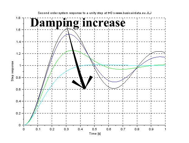
Modeling the dynamics of the wind vane a second-order system as model, we end up with two significant parameters of the system:resonance frequencyanddamping. Initially, bearing and other sources of friction on the main shaft will be neglected. A known resonance frequency value is used to verify that the wind vane is not excited by other mechanical devices, as depicted in the previous part. Wind gusts are generally an intended source of AoA readings, but we must ensure that their frequency content does not approach nor exceed the resonance frequency, so as the frequency response of our system has unity magnitude. Damping indicates how faster an excited oscillation decreases with time. The following picture illustrates the time response of a second-order system, while varying the value of damping. Our wind vane will be underdamped, hence its damping value will lie withing the (0,1) range.
The following equation defines a second-order transfer function using common notation. Since our vane will be underdamped, the typical time response will be oscillatory, with an exponential time decay term which reduces the oscillation magnitude in time.
is the natural frequency
or zeta is the damping
Equation AOA 1 - Standard second-order transfer function. Transfer function DC gain is equal to one.
is the damped frequency, oscillation in time occur at this frequency
Equation AOA 2 - Damped frequency definition
Figure AoA 5a - Second order system step response
Damping values as follows Black 0,15, Blue 0,2, Green 0,4, Light blue 0,8.
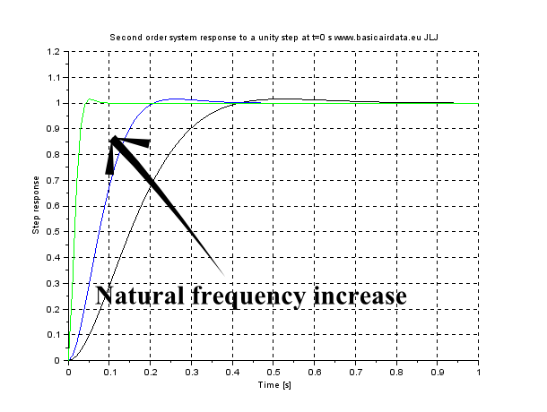
Figure AoA 5b - Second order system step response
Natural frequency value as follow Black 10, Blue 20,Green 100.
Inspection of the previous figures reveals that for good system behaviour (fast and stable measurements) we need a high value for both resonance frequency and damping. A SciLab file available for experimenting with parameter values can be found here. To increase wind vane resonance frequency, much like many mechanical systems, inertia decrease is required. Our wind vane is statically balanced with a fore mass and the overall weight can be decreased by enlarging the distance of the counterweight and decreasing the distance of the fin from the rotation axis of the vane. On the other hand, using a long fin arm will increase the damping of the system which is an also desirable characteristic, as is also describedhere, eq.6.
Thus, we end up with two conflicting requirements in our design phase. If an extremely fast dynamic response is needed, the ideal design is a leading edge wind vane, which is a vane that pivots directly in the leading edge of the fin, with no counterweight. If high values of damping are required, the classical long-armed wind vane is more promising. Since there is no dominant argument when choosing those values, a value greater than 0,15 is a good start, in order to avoid uncontrolled oscillations during operation. A damped system oscillates at the damped frequency
Wd of eq.2, as per figure AoA 5b.
When damping is low, the damped frequency value is close to the natural frequency. Natural frequency should be two times the maximum frequency of the measured quantity, in order to ensure unity measurement gain. Also, as has been said in the previous post, vane resonance frequency should be lower than 0.7 times the Airboom resonance value, or at least, this is a good first estimate; the more distance between the two resonance frequencies the better.
In a typical operating scenario, the vane will have to deal with a constant wind, with gusts superimposed on it. For design and simulation purposes gust models are available, such as the Dryden,FARandFAR2models. Wind gust library blocks also exist in many simulation packages.
Triggered by some chat around the net I post here some material about mechanical wind vanes design.
Angle of attack measurement by means of wind vanes will be first introduced. The topics to be covered in this miniseries are design, practical issues and modeling.
Angle of attack (AoA) instruments measure the angle between the airspeed vector and a predefined line on a cross-section of the airplane wing. This line is usually selected either as the zero-lift line or the chord line of the airfoil. AoA is often indicated by the Greek letter alpha. This angle is often used to calculate the lift of said wing section. AoA vanes are also called alpha vanes.
AoA usually changes across the wingspan of the aircraft and this is something one should take into account. A visual example is a wing which twists progressively across its span, flying straight and level. The AoA at the wing root differs from the AoA at the wing tip by the wing geometric twist term.
AoA measurements are are useful for parameter identification, general aviation planes or even to FPV pilots of RC-aircraft, since they can be used as an early warning indication as the vehicle approaches stall. The use case affects the choice of the AoA sensor type and desired performance. There are many types of AoA measurement devices, of which the most common are:
Wind vanes;
Null seeking devices;
Static-type devices, based exclusively on pressure measurement.
For a general description of these typologies, please refer to NACA-TN-4351.
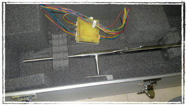
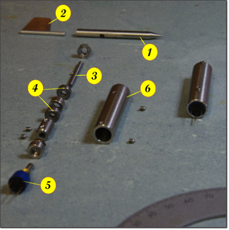
In this section we will focus on a classic mass-balanced wind vane design. Even though it is less attractive than a pressure-based unit or closed-loop null seeking device. Making and calibrating a good wind vane is well-withing the reach of a DIY maker. The wind vane visible below is made by Basic Air Data members and visualizes the main components of the system. A rendering of the completed assembly of the vane can be seen in figure AoA 2.
Equally important to the instrument itself, is the definition of the quantity under measurement: an adequate design requires stating specifications beforehand. Initially, our focus will be turned towards common design aspects and then some specifications will be proposed. A lot of bibliography can be found regarding weather vanes specifically; in principle, it's a valuable resournce but not very helpful when it comes to design requirements.
There are two main macroscopic differences between weather vane and alpha vane applications: range of speeds and the vane support structure, which is needed to isolate the instrument from vibrations degrading measurment quality. Imagine a wind vane fixed on a cantilever beam. In such configuration, which resembles a nose-mounted airboom, the whole structure may start to oscillate. As a case study, we will consider a planar oscillation (ref eq.36).
Given the height of the wind vane mounting point, h, and its airspeed, u, the error angle caused by beam deflection can be calculated as:
Given an airspeed of 20 m/s and a maximum deflection of 20 mm at 10 Hz, the error is:Another issue to be taken into account is that the motion of the mount at the
wind vane mounting point can interact with the wind vane dynamics. To avoid performance degradation it is crucial to maintain the resonant frequencies of the two systems well apart.
Since the air-boom doesn't have a simple geometry, the calculation of the vibration modes is not feasible using a closed form formula.
A 3D model needs to be created in a computing environment and FEM modal analysis be carried out. Alternatively, lab tests are also a way to obtain such data. Figure AoA 3 depicts the first mode of the probe. Elmer is a notable open FEM package that can be freely downloaded and can handle dynamic analysis.
Generally speaking, the stiffer the airboom, the higher its first resonant frequency will be. Higher airboom resonant frequencies are desirable, since they present an uppper performance limit for the wind vane. As a rule of thumb, if the airboom assembly moves under a slight force of the hand while while fixed on the ground, some vibration-related problems are to be expected.
More accurately, if numerical analysis tools is available, make sure that the first resonant frequency of the airboom is far from the desired wind vane operational range. An offset of at least 0.3 times the first mode frequency is a good, conservative value.
Resonant frequencies of higher order can be usually neglected, as they carry significantly less deflection energy. For best performance, it is always a good idea to make sure that to other vehicle components create excitations in the low to mid frequencies of the wind vane.
Let's proceed by examining wind vane behavior; refer to figure AoA 1.
The most critical component are the bearing. A Coulomb friction model will be used to describe their static friction.
The phenomenon of static friction, or stiction, results in the torque that is necessary to start rotating a resting bearing being greater than the torque required to keep it rolling. A graph representation of this phenomenon is found in figure AoA 4. This non-linearity leads to some problems when it is incoroporated in numerical integration algorithms.
Firstly, longer integration calculation times are to be expected. Furthermore, limit cycles and solution collisions may be generated, in other words the solution may be non-steady/cyclic or converge to a terminal value that yields a non zero static tracking error.
Analysis can become much neater if the model is writen down as a Filippov system: a nice, sliding bifurcation arises.
Figure AOA 2 - Miniature DIY Wind Vane 3D model (JLJ and GC)
Figure AoA 3 - Modal analysis on the probe, first mode frequency is 106Hz.
The probe is fixed at the root. The Maximum deflection at the tip 3 is 25 mm, 16 mm at the 2 windvane fixation point and 0 mm at the root 1.
Figure AoA 4 - Bearing friction model including stiction
Many articles are available on the wind vane topic, for example: J. Wieringa (1967), Evaluation and Design of Wind Vanes, Royal Netherlands Meteorological Institute, De Bilt (Download link)
Commonly, the vane dynamic behavior, at least near equilibrium, can be assimilated as one of a second order underdamped system. Standard industrial methods for determining the dynamic performance of a wind vane also exist, for example ASTM—D5366 “Standard Test Method for Determining the Dynamic Performance of a Wind Vane”.
I report some of the work that I/We did, within a Open Project, on a removable Pitot Flange.
After some "design-fix-test" iterations the new removable Pitot flange passed the pressure test; test pressure was 8 barg.
You find the free downloadable 3D models on GitHub.
Have a look to the following general arrangement drawing.
Figure 1 FF-8-500 - Front Flange for 8 mm Pitot- Assembly – 20141025
Major concern was the possible leaking of the pressure lines; sealing is attained with o-rings.Test consisted in pressurize the total pressure and the static pressure line. Pressure was applied at one line per time or on both lines at the same time. You can see the unit under test in figure 2.
Figure 2 Flange under test
The new flange is suitable to be used with the new air data computer, assembly view in figure 3. Flange connected by means of two pressure ports or lines; one port is for the total pressure that is routed from the probe tip and the other for the static pressure.
Figure 3 Removable Flange, Pitot and Air Data Computer, all from BAD Open Project
As the flange is equipped with push-in pneumatic fittings the pressure vessel is also connected with push-in fittings; you can see the coupling detail on figure 4.
Figure 4 Push-in pneumatic fittings and coupling
Refer to figure 5.The main part of the test equipment consist in a pressure vessel. Within this vessel the pressure is adjustable by mean of a valve connected to an air compressor. On the same pressure vessel is fixed a manometer. To test a pressure line we reach the desired test pressure and then we wait 15 minutes. If after that lapse of time the manometer indication is still the same then the test for this port and pressure is considered passed.
Figure 5 Test equipment
The maximum expected operating pressure is about 1,3 barg, the test pressure was set to two times operating pressure or 2.6 barg. As the results of test were positive at 2.6 barg we decided to push further. We tested the flange up to 8 barg.
I've just updated a little set of Android Apps that are useful in many telemetry related issues. The main reference page is http://www.basicairdata.eu/mobile.html .
The apps are free and open source, part of BasicAirData Project. Calculations algorithms documented.
GPSLogger; It is a straight forward GPS Logger; It corrects the altitude measurements with NASA EGM model.


